DistributionRegressor

California Housing (vs NGBoost)

Predicting the full house value distribution conditional on location and census features (8 features, 20,640 samples). Compared against NGBoost on test-set negative log-likelihood.

Benchmark results

The limitation of parametric models

NGBoost with a Normal distribution forces every prediction into a symmetric, unimodal bell curve. When the true conditional distribution is multimodal, skewed, or bounded, the parametric assumption breaks down and wastes probability mass on impossible values.

NGBoost can use more complex parametric families to mitigate this, but the user must choose the right family in advance. DistributionRegressor sidesteps this entirely - it learns whatever shape the data requires.

Monte Carlo Training (monte_carlo_training)

By default, the training set is expanded to n_samples × n_bins rows: every sample is paired with every grid point. Monte Carlo training instead samples mc_samples uniform grid points per sample, reducing peak memory significantly. With periodic resampling (mc_resample_freq), different groups of trees train on different random grid points, improving coverage of the threshold space.

How it works

For each training sample, mc_samples threshold points are drawn uniformly from the grid range. The mc_resample_freq parameter controls how often fresh points are drawn:

• mc_resample_freq=100 (default): Resample every 100 trees. With 1000 trees, the model trains on 10 different random grids. Low overhead.
• mc_resample_freq=10: Resample every 10 trees. More grid coverage, but higher overhead from repeated dataset construction and LightGBM init_model calls.

Resampling works via LightGBM's incremental training (init_model): each group of trees continues from the previous model but trains on a freshly sampled expanded dataset. The idea is analogous to mini-batch SGD — each batch of trees sees a different random slice of the threshold space.

Memory comparison

When to use it

MC training is useful when full grid expansion would exceed available memory — typically with large training sets (100k+ samples) and high n_bins (100+). For small to medium datasets, the full grid is simpler and fast enough.

Resampling (mc_resample_freq) significantly improves MC quality compared to single-shot MC. In our benchmarks on the Rossmann dataset, MC with mc_resample_freq=10 produced distributions visually close to the full grid, with comparable NLL. Results may vary by dataset — we recommend comparing on your own data.

# Full grid (default) - simple, good for small/medium datasets
model = DistributionRegressor(n_bins=100)

# MC with resampling - for large datasets where memory is tight
model = DistributionRegressor(
    monte_carlo_training=True,
    mc_samples=20,
    mc_resample_freq=100,   # resample grid points every 100 trees
    n_bins=100,
)

# MC with frequent resampling - better grid coverage, more overhead
model = DistributionRegressor(
    monte_carlo_training=True,
    mc_samples=20,
    mc_resample_freq=10,    # resample every 10 trees
    n_bins=100,
)

Quality comparison

The chart below compares the full grid against MC with two resampling frequencies on the Rossmann dataset. With mc_resample_freq=10, MC closely tracks the full grid distributions:

Tuning Guide

Practical guidance for getting the best results from DistributionRegressor.

Step 1: Start with good defaults

For most problems, the following configuration works well out of the box:

model = DistributionRegressor(
    n_bins=100,
    n_estimators=1000,
    learning_rate=0.01,
    random_state=42,
)

Step 2: Adjust n_bins for your target range

n_bins controls the resolution of the predicted distribution. Think of it as the number of "buckets" the model uses to represent the density.

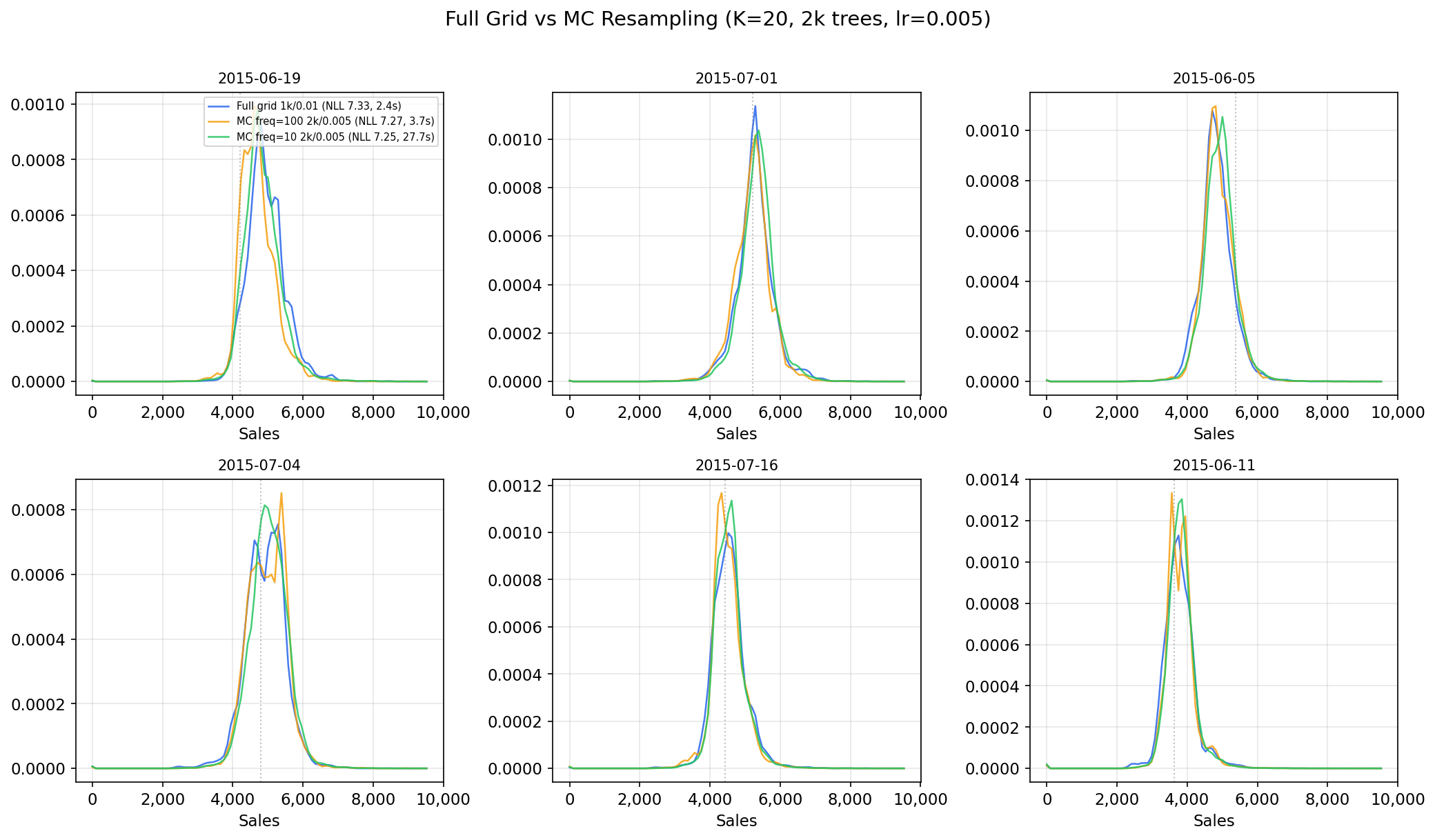
Higher n_bins gives finer resolution but increases memory linearly. If memory is tight, combine higher n_bins with monte_carlo_training=True and mc_resample_freq (see Monte Carlo Training).

Step 3: Tune the LightGBM parameters

Since DistributionRegressor uses LightGBM under the hood, all standard LGBM tuning strategies apply. Pass any parameter through **kwargs:

model = DistributionRegressor(
    n_bins=100,
    n_estimators=1000,
    learning_rate=0.01,
    # Standard LightGBM parameters
    num_leaves=63,
    max_depth=-1,
    subsample=0.8,
    colsample_bytree=0.8,
    min_child_samples=20,
)

Step 4: Evaluate with proper scoring rules

Use negative log-likelihood (NLL) as your primary evaluation metric for the distribution quality. Lower NLL means better-calibrated, sharper distributions. Use RMSE or MAE alongside NLL to evaluate point prediction quality:

# Distribution quality (proper scoring rule)
nll = model.nll(X_test, y_test)

# Point prediction quality
from sklearn.metrics import mean_squared_error
rmse = mean_squared_error(y_test, model.predict(X_test), squared=False)

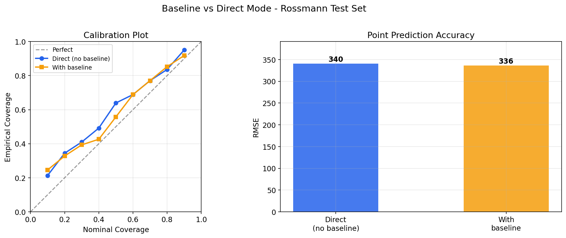
# Calibration check: does 90% interval contain ~90% of true values?
iv = model.predict_interval(X_test, confidence=0.9)
coverage = ((y_test >= iv[:, 0]) & (y_test <= iv[:, 1])).mean()
print(f"90% interval coverage: {coverage:.1%}")

Step 5: Apply output smoothing if needed

If the predicted densities look too jagged (especially at lower n_bins), apply Gaussian smoothing. You can experiment with this after training without refitting:

# Try different smoothing levels
for sigma in [0, 0.5, 1, 2]:
    model.set_output_smoothing(sigma)
    nll = model.nll(X_test, y_test)
    print(f"sigma={sigma}: NLL={nll:.4f}")

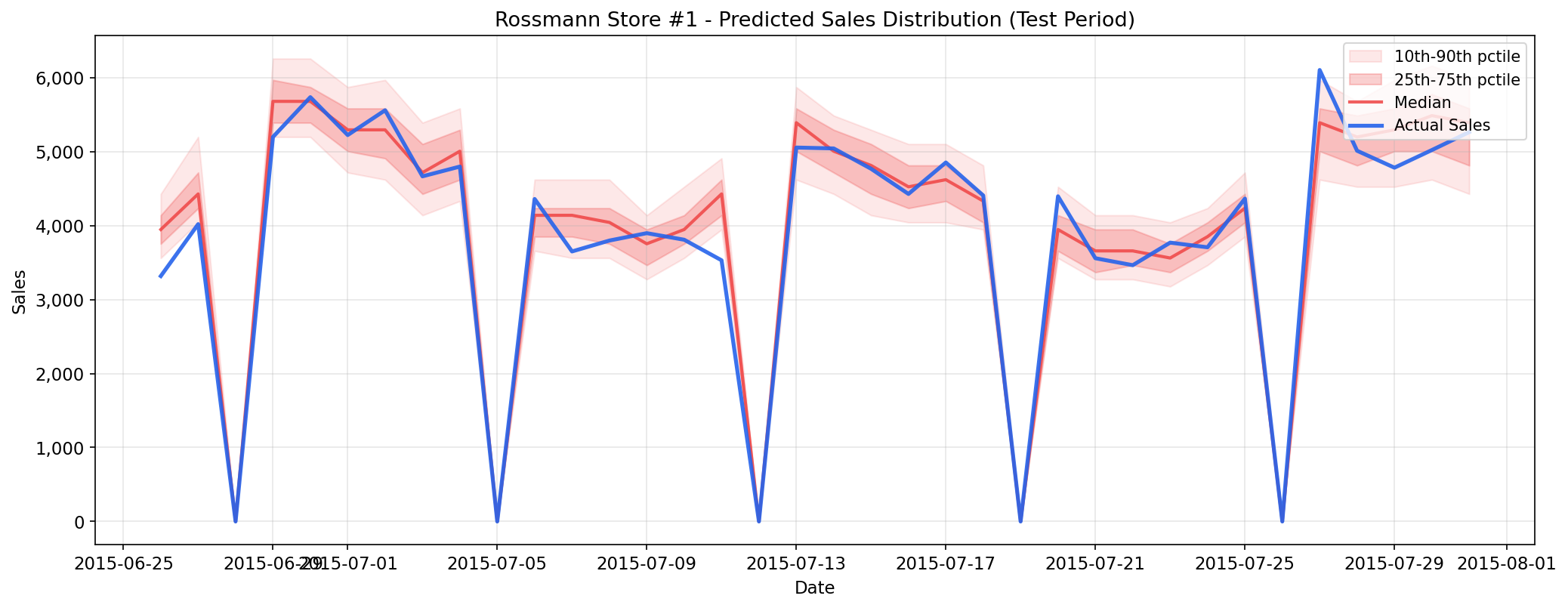
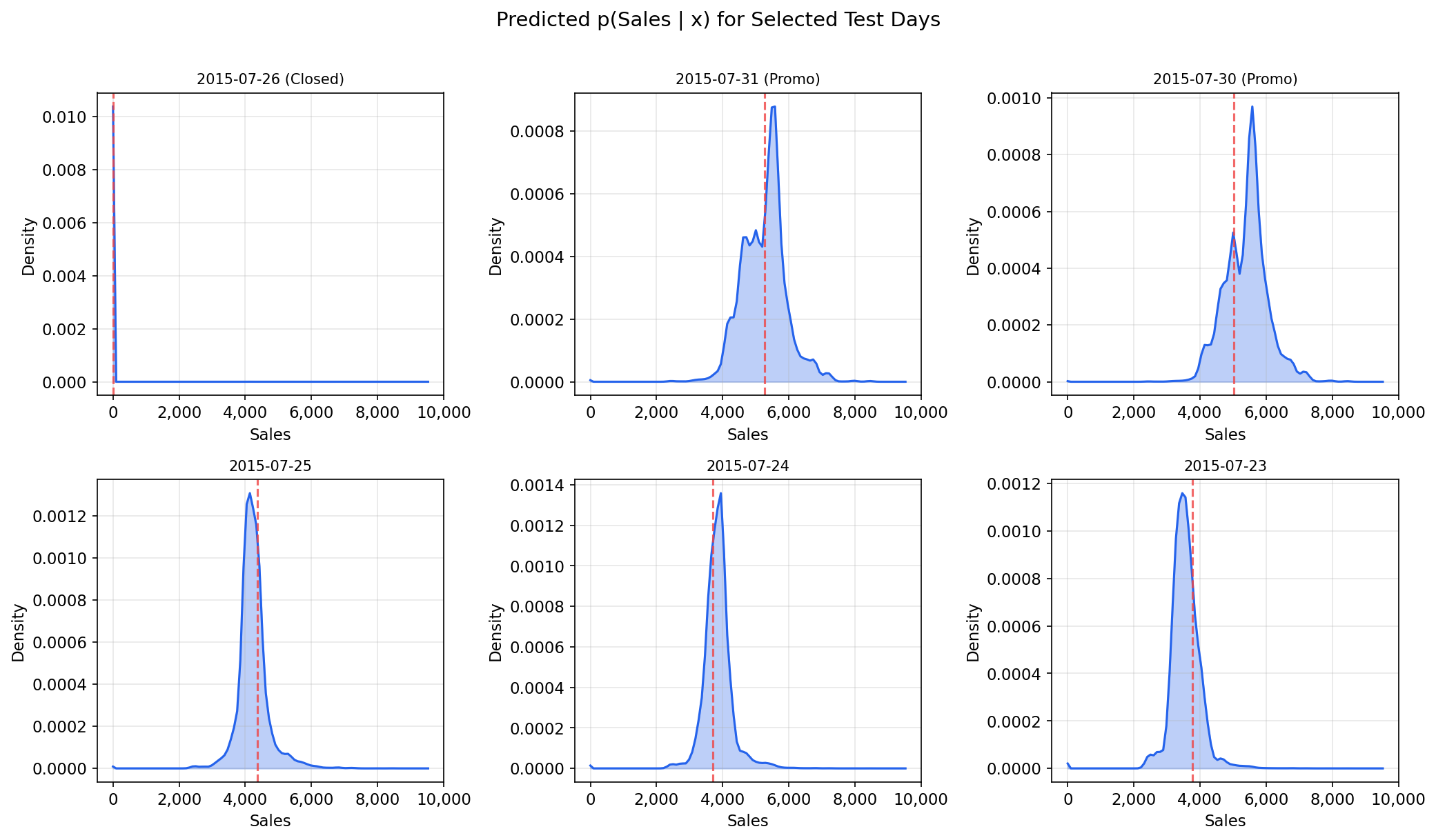
# If target has discrete atoms (e.g., exact zeros), preserve them
model.set_output_smoothing(output_smoothing=1, atom_values=0)