FuzzyDTree

Decision trees with smooth fuzzy splits for regression and classification — interpretable, smooth, and sklearn-compatible.

$ pip install FuzzyDTree

Regressor Classifier API

Standard decision trees produce jagged, discontinuous predictions. Small changes in input can cause a sample to jump between completely different leaf nodes. FuzzyDTree replaces hard thresholds with smooth compact-support membership functions, so each sample partially belongs to multiple leaves.

Aspect	Hard Decision Tree	Fuzzy Decision Tree
Split function	`x ≤ threshold ? left : right`	`μ(x) = S((x - threshold) / margin)`
Sample routing	Goes to exactly one leaf	Partially belongs to multiple leaves
Prediction surface	Piecewise constant (step functions)	Smooth, continuous transitions
Sensitivity to thresholds	Discontinuous at every split boundary	Gradual transition controlled by margin

How Fuzzy Splits Work

At each split node, instead of a hard left/right decision, a compact-support S-curve assigns a continuous degree of belonging to each child. The transition width (margin) is learned per split from a data-driven geometric grid.

1. Split Candidate

Feature j, threshold t

→

2. Margin Selection

Try geometric grid of margin values
from 0.4·std to 20·std

↓

4. Weighted Average

Prediction = Σ μ_leaf · v_leaf

←

3. Membership

μ_left = S((x−t)/margin)
μ_right = 1 − μ_left

Interactive: Fuzzy vs Hard Split

Drag the margin slider to see how the transition width controls fuzziness. At margin→0, the S-curve becomes a hard step function (standard tree). Outside [threshold−margin, threshold+margin] the membership is exactly 0 or 1.

Threshold (t): 0.50

Margin (m): 0.10

Small margin → crisp split
Large margin → smooth, fuzzy transition

Package Components

The package exposes two estimators plus a small set of inspection utilities. Both estimators follow the scikit-learn estimator interface and share the same tree-building machinery.

Component	Type	Purpose	Main methods / attributes
`FuzzyTreeRegressor`	Estimator	Single-tree regression with fuzzy numeric splits and optional joint leaf-value refit.	`fit`, `predict`, `score`, `feature_importances_`
`FuzzyTreeClassifier`	Estimator	Single-tree classification with fuzzy numeric splits and class-probability predictions.	`fit`, `predict`, `predict_proba`, `classes_`
`plot_tree()`	Inspection method	Matplotlib rendering of split nodes, thresholds, margins, sample counts, and leaf values.	Available on fitted estimators
`explain_prediction()`	Inspection method	Per-sample explanation containing reached leaves, path weights, and feature contributions.	Available on fitted estimators
`plot_feature_contributions()`	Inspection method	Waterfall plot for the output of `explain_prediction()`.	Available on fitted estimators

Shared Mechanics

Area	Implementation
Numeric splits	Threshold and margin candidates are evaluated on pre-binned features using Numba-compiled kernels.
Membership function	Compact-support quadratic S-curve, controlled by a per-split margin.
Missing values	NaN routing direction is selected during split search and stored on the fitted node.
Categorical features	Optional categorical handling with binary partitions; columns can be supplied explicitly or auto-detected.
scikit-learn compatibility	`get_params` and `set_params` are implemented for estimator composition and model selection.

FuzzyTreeRegressor

A single-tree regressor with smooth compact-support fuzzy splits. Produces continuous prediction surfaces while remaining fully interpretable — you can visualize the tree, inspect feature importances, and explain individual predictions.

Quick Start

from fuzzydtree import FuzzyTreeRegressor
from sklearn.datasets import fetch_california_housing
from sklearn.model_selection import train_test_split

X, y = fetch_california_housing(return_X_y=True)
X_train, X_test, y_train, y_test = train_test_split(X, y, random_state=42)

model = FuzzyTreeRegressor(max_depth=8)
model.fit(X_train, y_train)

y_pred = model.predict(X_test)
print(f"R² = {model.score(X_test, y_test):.4f}")

How It Differs from sklearn

sklearn DecisionTreeRegressor

Hard threshold: x ≤ t
Each sample reaches exactly one leaf
Piecewise constant surface
Discontinuities at every split boundary

FuzzyTreeRegressor

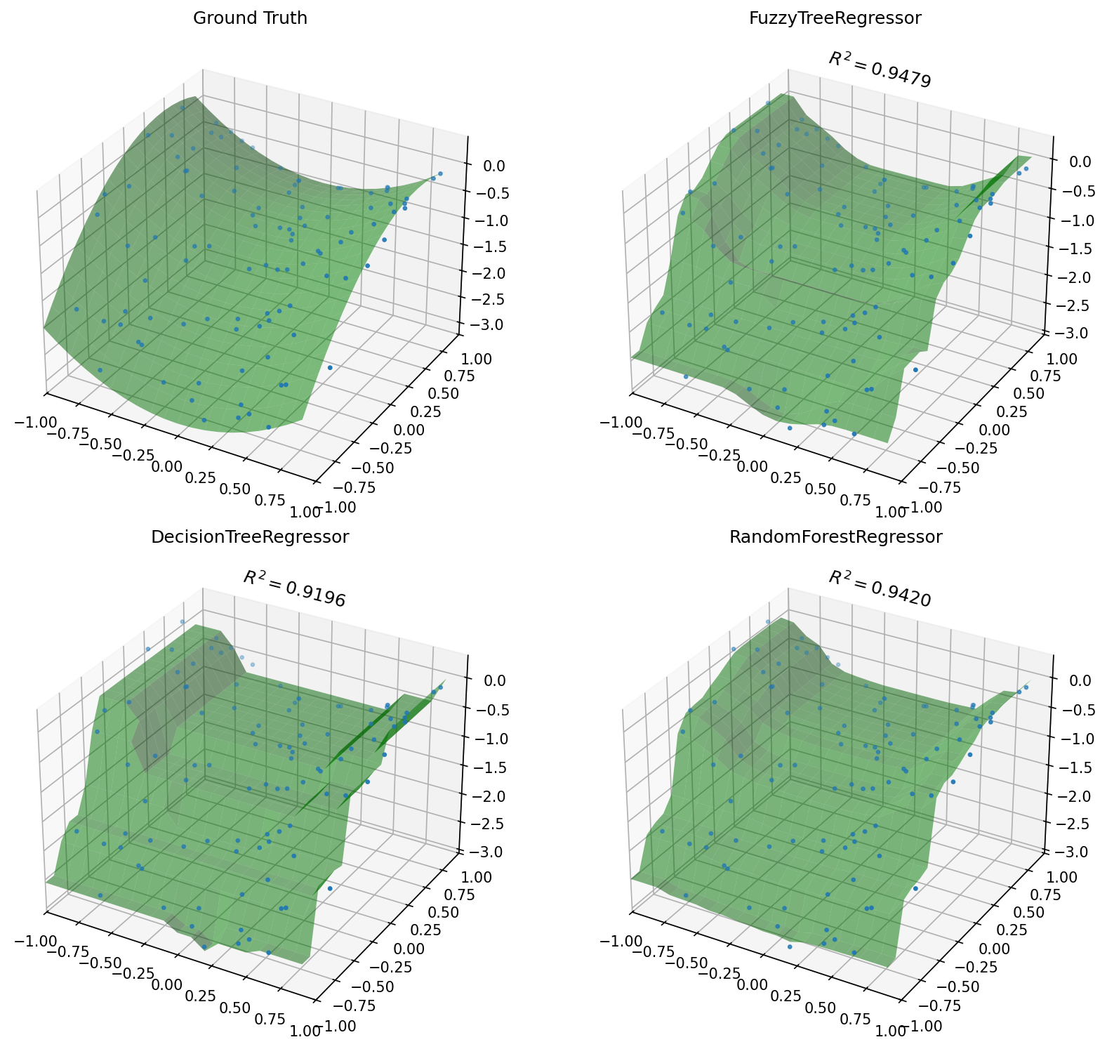
S-curve membership: μ = S((x−t)/margin)
Each sample reaches multiple leaves with different weights
Smooth, continuous surface
Gradual transition controlled by learned margin

Example 1: Synthetic Decision Surface

Synthetic 2D function: y = X₀² − X₁² + X₁ − 1. 100 training points from [-1, 1]². Comparison with sklearn DecisionTree and RandomForest.

from fuzzydtree import FuzzyTreeRegressor
from sklearn.tree import DecisionTreeRegressor
from sklearn.ensemble import RandomForestRegressor

est_fuzzy = FuzzyTreeRegressor(max_depth=5, optimize_leaf_values=True, leaf_l2=0.1)
est_fuzzy.fit(X_train, y_train)

est_tree = DecisionTreeRegressor(max_depth=5)
est_tree.fit(X_train, y_train)

est_rf = RandomForestRegressor(n_estimators=100, max_depth=5, random_state=0)
est_rf.fit(X_train, y_train)

        Results:

        FuzzyTreeRegressor R² = 0.949 (leaves=24, depth=5)

        DecisionTreeRegressor R² = 0.920

        RandomForestRegressor R² = 0.942

Decision surface comparison: FuzzyTreeRegressor vs sklearn DecisionTree vs RandomForest

Decision surfaces on y = X²⊂0 − X²⊂1 + X⊂1 − 1. FuzzyTreeRegressor produces a smoother surface than a hard tree, beating a 100-tree random forest with a single tree.

Feature Importances

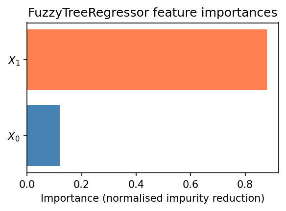
imp = est_fuzzy.feature_importances_
# X0: 0.xxx   X1: 0.xxx

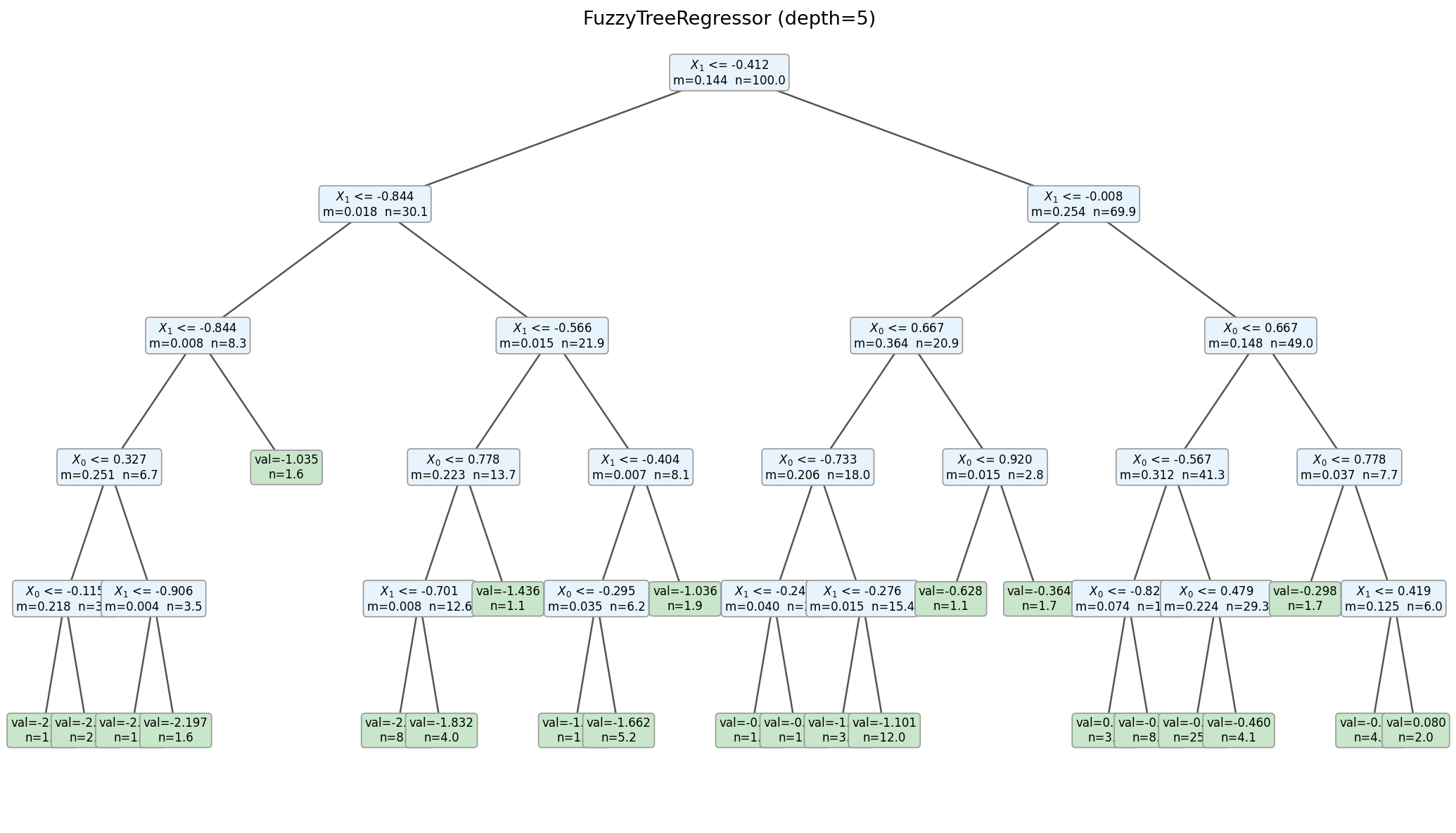
Feature importances on the 2D synthetic function showing both features contribute meaningfully.

Tree Structure

Inspect the learned tree structure including split features, thresholds, margin values, and leaf predictions.

fig, ax = plt.subplots(figsize=(14, 8))
est_fuzzy.plot_tree(feature_names=['$X_0$', '$X_1$'], ax=ax, fontsize=8)
plt.show()

Fuzzy decision tree structure visualization

Tree structure showing split nodes (blue) with feature, threshold, and margin values, and leaf nodes (green) with predicted values.

Example 2: California Housing

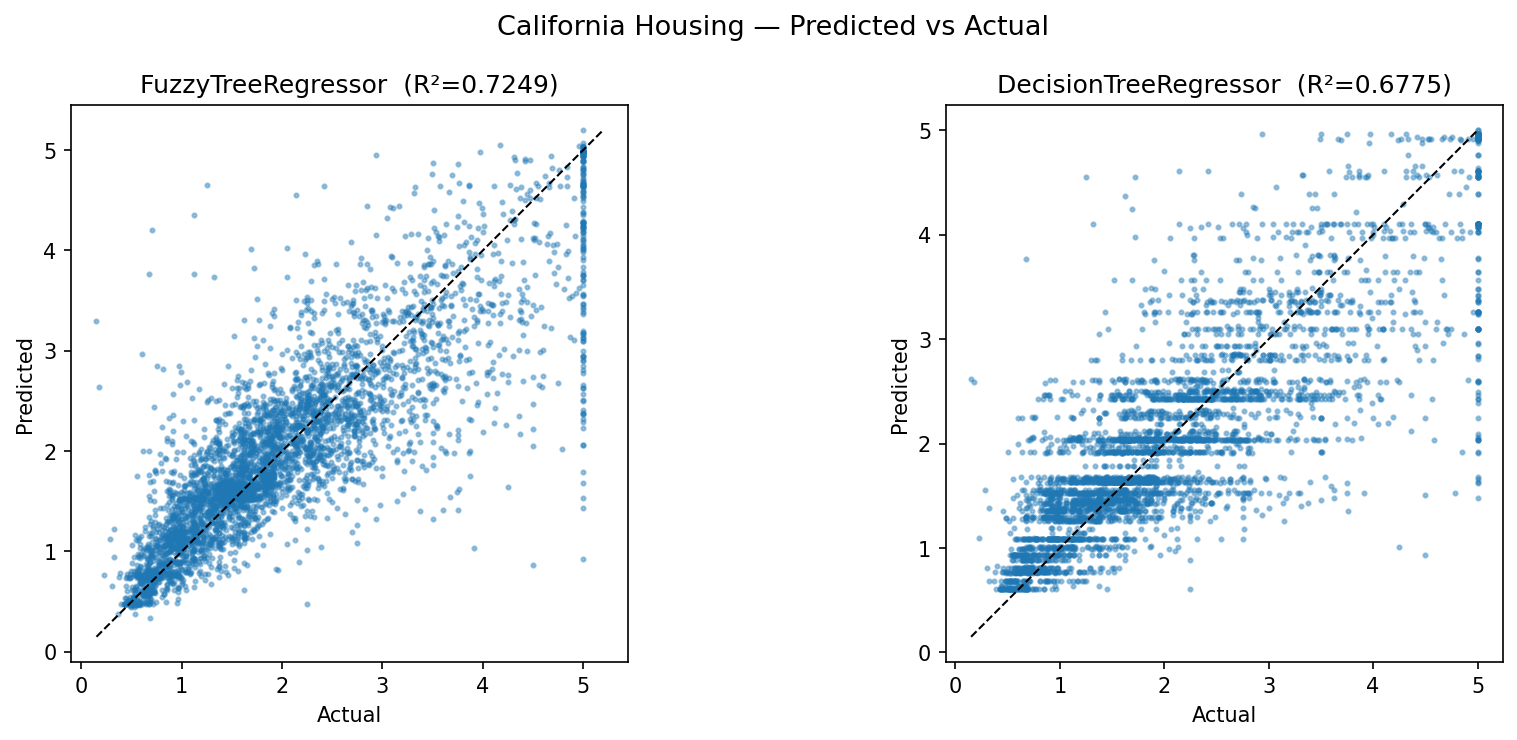
Predicting median house value (in $100k) from the California Housing dataset (20,640 samples, 8 features). No external data needed — sklearn downloads it automatically.

from fuzzydtree import FuzzyTreeRegressor
from sklearn.datasets import fetch_california_housing
from sklearn.model_selection import train_test_split

data = fetch_california_housing()
X_tr, X_te, y_tr, y_te = train_test_split(
    data.data, data.target, test_size=0.2, random_state=42)

model = FuzzyTreeRegressor(max_depth=8, optimize_leaf_values=True)
model.fit(X_tr, y_tr)
print(f"R² = {model.score(X_te, y_te):.4f}")

Predicted vs Actual

FuzzyTreeRegressor vs DecisionTreeRegressor on California Housing. The fuzzy tree produces tighter scatter around the diagonal.

Feature Contribution Waterfall

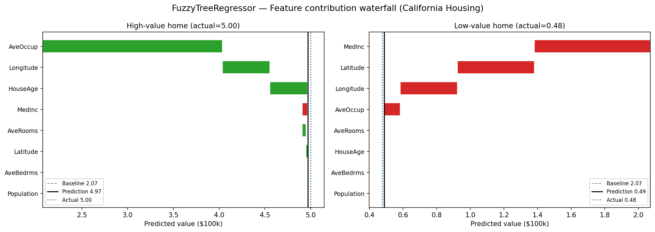
plot_feature_contributions() visualises how each feature pushes the prediction away from the baseline (training mean). Green bars push up, red bars push down.

# Built-in waterfall plot
model.plot_feature_contributions(
    X_te[idx],
    feature_names=data.feature_names,
    actual=y_te[idx]
)

High-value vs low-value home. Each bar shows a feature's contribution from the baseline to the final prediction. Dashed lines: baseline, prediction, actual.

Parameters

Parameter	Default	Description
`max_depth`	5	Maximum depth of the tree.
`max_leaves`	None	Maximum leaf nodes. Enables best-first growth when set.
`min_samples_leaf`	1.0	Minimum effective (weighted) sample count per child for a split to be accepted.
`max_features`	None	Features considered per split. `None` = all. Accepts `'sqrt'`, `'log2'`, int, or float.
`margin_grid_size`	10	Number of margin candidates in the geometric grid per split.
`max_bins`	256	Maximum histogram bins for threshold candidates.
`min_train_weight_fraction`	0.01	Minimum relative training weight retained when propagating fuzzy child weights.
`prebin_numeric`	True	Pre-bin numeric features once before split search for faster histogram-based training.
`margin_depth_decay`	1.0	Exponential decay factor for the margin upper bound at each depth level.
`optimize_leaf_values`	True	Re-solve all leaf values jointly via weighted least-squares after tree construction. Produces substantially better predictions.
`optimize_split_gain`	False	Use exact fuzzy two-leaf least-squares objective for split evaluation instead of the faster weighted child-mean approximation.
`leaf_l2`	0.1	L2 regularization for the joint leaf-value solve.
`categorical_features`	None	Indices of categorical columns, or `'auto'` for automatic detection.
`max_cat_threshold`	64	Maximum number of unique values for a feature to be auto-detected as categorical.
`random_state`	None	Random seed for reproducibility when using feature subsampling.

FuzzyTreeClassifier

A single-tree classifier with smooth compact-support fuzzy splits and logit-MSE/Gini split selection. Produces smooth decision boundaries and calibrated class probabilities while remaining fully interpretable.

Quick Start

from fuzzydtree import FuzzyTreeClassifier
from sklearn.datasets import make_moons
from sklearn.model_selection import train_test_split
from sklearn.preprocessing import StandardScaler

X, y = make_moons(n_samples=300, noise=0.25, random_state=0)
X = StandardScaler().fit_transform(X)
X_train, X_test, y_train, y_test = train_test_split(X, y, test_size=0.3, random_state=42)

clf = FuzzyTreeClassifier(max_depth=5)
clf.fit(X_train, y_train)

print(f"Accuracy = {clf.score(X_test, y_test):.1%}")
probs = clf.predict_proba(X_test)  # shape: (n_samples, n_classes)

How It Differs from sklearn

sklearn DecisionTreeClassifier

Hard threshold: x ≤ t
Piecewise constant class probabilities
Rectangular decision regions
Probability = fraction of leaf samples

FuzzyTreeClassifier

S-curve membership: μ = S((x−t)/margin)
Smooth probability gradients across boundaries
Curved, non-rectangular decision regions
Probability = weighted mix of leaf distributions

Example 1: Classification Benchmarks

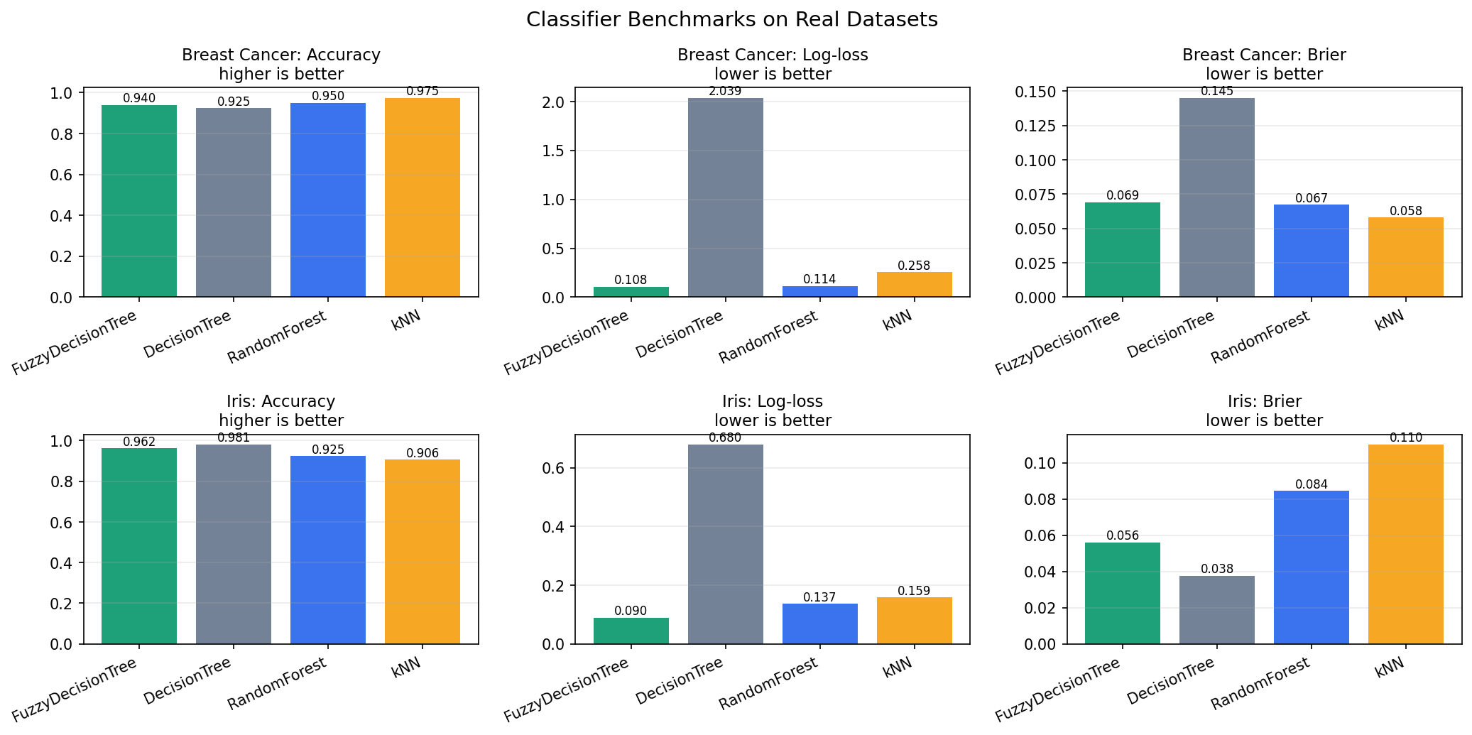
Breast Cancer and Iris provide binary and multiclass tabular classification examples. The comparison reports held-out accuracy plus probability metrics for predict_proba.

from sklearn.datasets import load_breast_cancer, load_iris
from sklearn.metrics import accuracy_score, log_loss

clf = FuzzyTreeClassifier(
    max_depth=5,
    min_samples_leaf=3,
    margin_grid_size=8,
    random_state=0,
)
clf.fit(X_train, y_train)

probs = clf.predict_proba(X_test)
pred = clf.predict(X_test)

        Key insight: FuzzyTreeClassifier provides competitive accuracy while
        retaining calibrated probability outputs from a single interpretable tree.
      

Classifier benchmark metrics on Breast Cancer and Iris

Held-out accuracy, log-loss, and Brier score on Breast Cancer and Iris. Lower is better for log-loss and Brier; higher is better for accuracy.

Example 2: Feature Contributions to Log-Odds

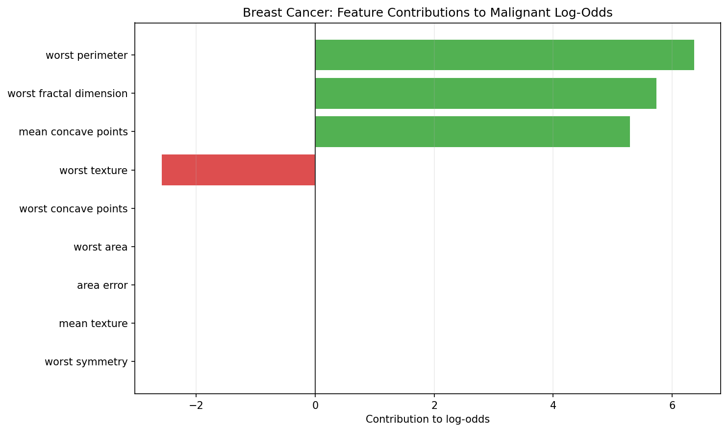
For classification, the most useful local explanation is often evidence for a class. explain_prediction_log_odds() decomposes the selected class probability into feature contributions in one-vs-rest log-odds, then converts the final log-odds back to probability.

exp = clf.explain_prediction_log_odds(
    X_test[i],
    class_label=0,  # malignant in sklearn's Breast Cancer dataset
    feature_names=data.feature_names,
)

print(exp["baseline_log_odds"], exp["prediction_log_odds"])
print(exp["prediction_probability"])

clf.plot_log_odds_contributions(
    X_test[i],
    class_label=0,
    feature_names=data.feature_names,
)

Classifier feature importances on Breast Cancer

Global feature importances for the Breast Cancer classifier, measured by normalized split-objective reduction.

Classifier log-odds feature contribution waterfall

Local explanation for a Breast Cancer prediction. Green bars increase the log-odds of the selected class; red bars decrease it. The title reports both final log-odds and probability.

Example 3: Multiclass Decision Boundaries on Iris

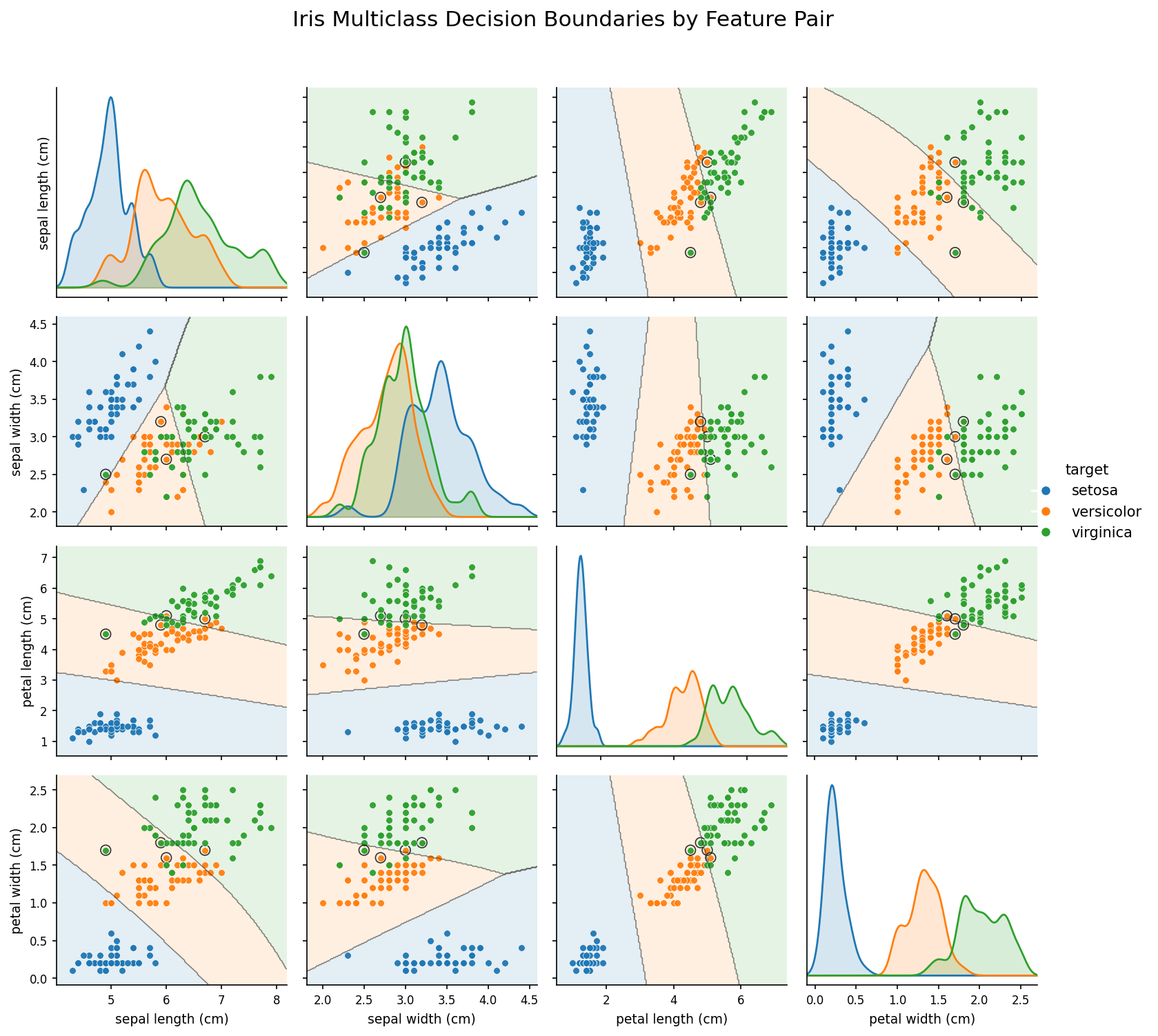
Iris is a compact three-class benchmark. The classifier handles multiclass labels directly, and each feature-pair panel below smooths the full-model predictions for the real Iris examples into a connected decision surface.

from fuzzydtree import FuzzyTreeClassifier
from sklearn.datasets import load_iris
from sklearn.model_selection import train_test_split

X, y = load_iris(return_X_y=True)
X_train, X_test, y_train, y_test = train_test_split(
    X, y, stratify=y, random_state=42)

clf = FuzzyTreeClassifier(max_depth=5)
clf.fit(X_train, y_train)

# predict returns class labels, predict_proba returns (n_samples, 3) array
labels = clf.predict(X_test)
probs  = clf.predict_proba(X_test)  # shape: (n_samples, 3)
score  = clf.score(X_test, y_test)

Iris pairplot with multiclass decision boundaries

Iris pairplot with density curves on the diagonal and full-model fuzzy multiclass decision regions in each feature-pair scatter panel. The background is a smoothed interpolation of the full model's per-example class probabilities.

Probability Surface

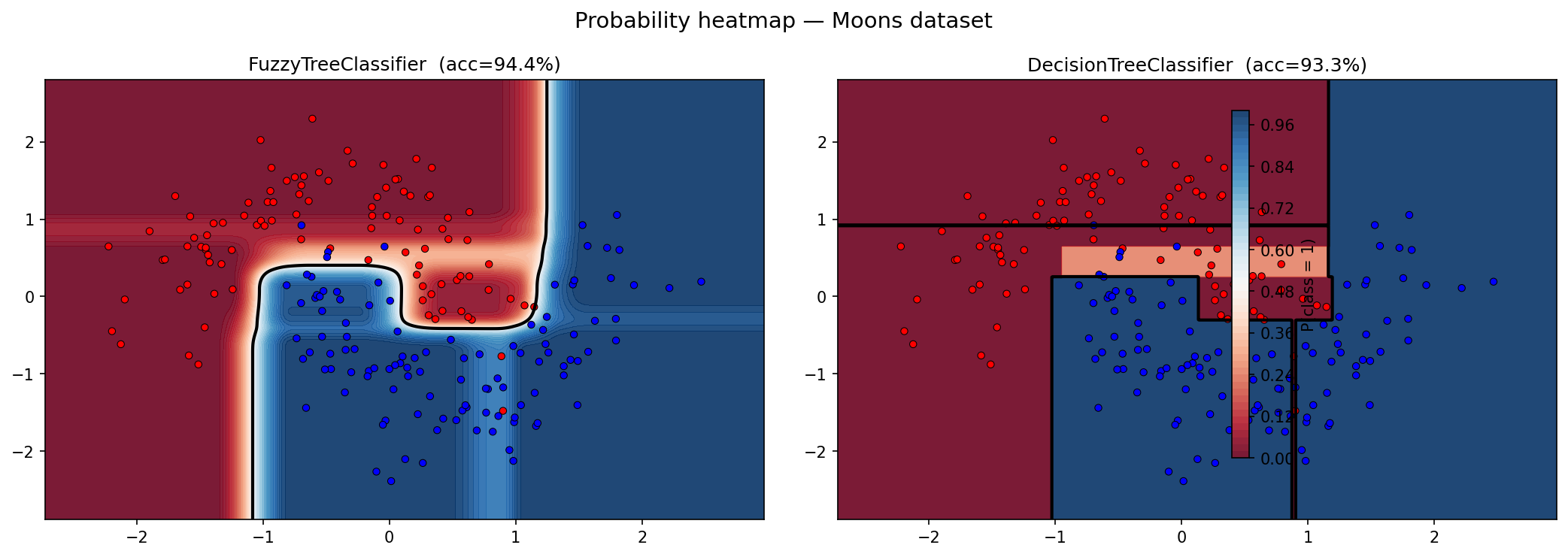
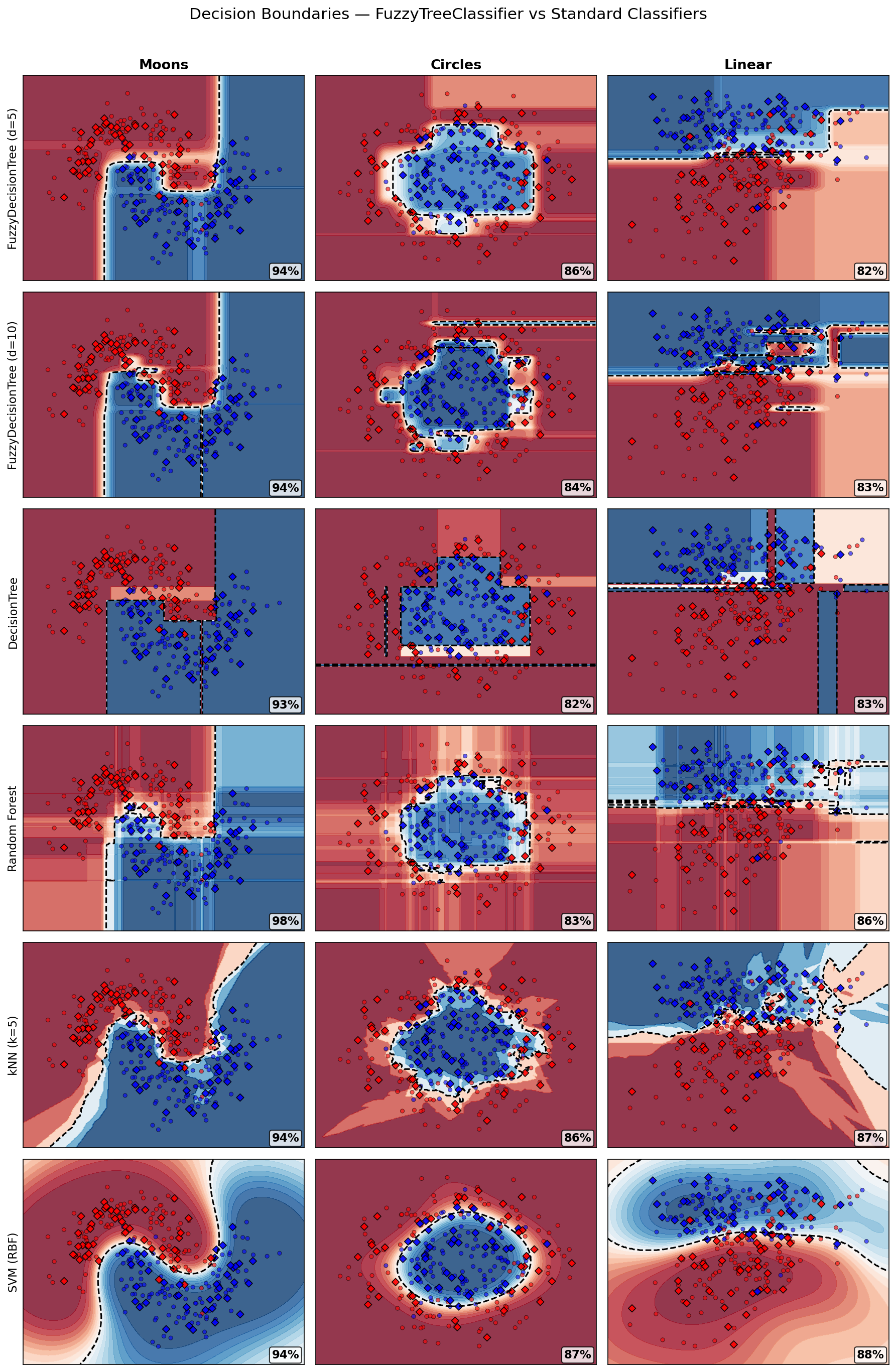
On two-dimensional datasets, fuzzy splits produce smooth probability transitions around decision boundaries instead of piecewise-constant rectangular regions.

Probability heatmap comparison: Fuzzy vs Hard tree

P(class=1) heatmap on the Moons dataset. The fuzzy tree produces a smooth probability gradient across the decision boundary; the hard tree produces sharp rectangular steps.

Decision boundary comparison across classifiers and datasets

Decision boundaries on two-dimensional classification datasets.

Parameters

The classifier accepts all base tree parameters (it does not use the regressor-specific optimize_leaf_values, optimize_split_gain, leaf_l2, leaf_l2_mode, split_gain_l2, refine_splits, refine_splits_max_iter, or refine_splits_candidates parameters):

Parameter	Default	Description
`max_depth`	5	Maximum depth of the tree.
`max_leaves`	None	Maximum leaf nodes. Enables best-first growth when set.
`min_samples_leaf`	1.0	Minimum effective (weighted) sample count per child for a split to be accepted.
`max_features`	None	Features considered per split. `None` = all. Accepts `'sqrt'`, `'log2'`, int, or float.
`margin_grid_size`	10	Number of margin candidates in the geometric grid per split.
`max_bins`	256	Maximum histogram bins for threshold candidates.
`min_train_weight_fraction`	0.01	Minimum relative training weight retained when propagating fuzzy child weights.
`prebin_numeric`	True	Pre-bin numeric features once before split search for faster histogram-based training.
`margin_depth_decay`	1.0	Exponential decay factor for the margin upper bound at each depth level.
`split_criterion`	`'logit_mse'`	Split objective. `'logit_mse'` and `'gini'` use the local least-squares finite-logit objective; `'entropy'` uses cross-entropy information gain.
`leaf_prediction`	`'frequency'`	Probability model. `'frequency'` uses fuzzy-weighted per-leaf class frequencies. Experimental alternatives: `'logit_mse'` and `'logit_ce'`.
`leaf_logit_l2`	0.01	L2 regularisation for logit leaf refits when `leaf_prediction` is a logit mode.
`leaf_logit_target`	4.0	Finite one-vs-rest target logit magnitude for `leaf_prediction='logit_mse'`.
`leaf_logit_ce_max_iter`	100	Maximum line-search iterations for `leaf_prediction='logit_ce'`.
`leaf_logit_ce_lr`	1.0	Initial line-search step size for `leaf_prediction='logit_ce'`.
`leaf_logit_ce_tol`	1e-6	Relative improvement tolerance for `leaf_prediction='logit_ce'`.
`categorical_features`	None	Indices of categorical columns, or `'auto'` for automatic detection.
`max_cat_threshold`	64	Maximum number of unique values for a feature to be auto-detected as categorical.
`random_state`	None	Random seed for reproducibility when using feature subsampling.

API Reference

Both models follow the sklearn estimator API. Methods are organized by model class.

FuzzyTreeRegressor

from fuzzydtree import FuzzyTreeRegressor

fit(X, y, sample_weight=None)

Train the fuzzy decision tree on features X and target y. Accepts optional sample_weight array. Returns self.

predict(X)

Predict target values. Returns array of shape (n_samples,). Each prediction is a weighted average over all reachable leaves.

score(X, y, sample_weight=None)

R² score on test data.

explain_prediction(x, feature_names=None)

Explain a single prediction. Returns dict with baseline, prediction, steps (per-split contributions), feature_contributions (aggregated by feature), and leaves (all reached leaves with value, weight, and path).

plot_tree(*, feature_names=None, ax=None, fontsize=9, node_color='#E8F4FD', leaf_color='#C8E6C9', edge_color='#555555')

Visualize the tree structure with matplotlib. Shows split features, thresholds, margin values, sample counts, and leaf predictions.

plot_feature_contributions(x, *, feature_names=None, actual=None, ax=None, positive_color='#2ca02c', negative_color='#d62728')

Waterfall chart of per-feature contributions for a single sample. Shows how each feature pushes the prediction away from the baseline (training mean). Optionally overlays the ground-truth value.

feature_importances_

Array of normalized impurity reductions per feature. Available after fit().

n_leaves_

Number of leaf nodes in the fitted tree.

depth_

Maximum depth reached in the fitted tree.

get_params(deep=True) / set_params(**params)

Sklearn-compatible parameter getters/setters.

FuzzyTreeClassifier

from fuzzydtree import FuzzyTreeClassifier

fit(X, y, sample_weight=None)

Train the fuzzy decision tree classifier on features X and labels y. Supports binary and multiclass classification. Returns self.

predict(X)

Return predicted class labels. Returns array of shape (n_samples,).

predict_proba(X)

Return class probabilities for each sample. Returns array of shape (n_samples, n_classes). Probabilities are computed from the fuzzy-weighted mixture of leaf class distributions.

predict_log_odds(X, class_label=None)

Return one-vs-rest log-odds for the selected class. For binary classification, the default selected class is the second class in classes_.

score(X, y, sample_weight=None)

Return mean accuracy on the given test data.

explain_prediction(x, feature_names=None)

Explain a single prediction. Returns dict with baseline, prediction, feature_contributions, and leaves (reached leaves with value, weight, and path).

explain_prediction_log_odds(x, *, class_label=None, feature_names=None)

Explain a selected class probability as feature contributions in one-vs-rest log-odds. Returns baseline probability/log-odds, final probability/log-odds, and per-feature contributions.

plot_tree(*, feature_names=None, ax=None, fontsize=9)

Visualize the tree structure with matplotlib.

plot_feature_contributions(x, *, feature_names=None, actual=None, ax=None)

Waterfall chart of per-feature contributions for a single sample.

plot_log_odds_contributions(x, *, class_label=None, feature_names=None, ax=None, max_features=10)

Waterfall chart of selected-class feature contributions in log-odds space.

feature_importances_

Array of normalized split-objective reductions per feature.

classes_

Array of unique class labels discovered during fit().

n_classes_

Number of classes.

n_leaves_

Number of leaf nodes in the fitted tree.

depth_

Maximum depth reached in the fitted tree.

get_params(deep=True) / set_params(**params)

Sklearn-compatible parameter getters/setters.

Examples

These examples are reproduced from the demo notebooks in the repository root. Run them yourself to generate the charts and explore the models interactively.

FuzzyTreeRegressor

Notebook: regressor_demo.ipynb

Decision Surface Comparison

Synthetic 2D function: y = X₀² − X₁² + X₁ − 1. FuzzyTreeRegressor (R²=0.949) produces a smooth surface that beats both a hard DecisionTree (R²=0.920) and a 100-tree RandomForest (R²=0.942).

Feature Importances

Normalized impurity reduction showing both features contribute to the quadratic surface.

Tree Structure Visualization

Split nodes (blue) show feature, threshold, and margin values. Leaf nodes (green) show predicted values and sample counts.

California Housing — Predicted vs Actual

FuzzyTreeRegressor vs DecisionTreeRegressor on California Housing (20k samples, 8 features).

Scatter around the diagonal is tighter for the fuzzy tree.

Feature Contribution Waterfall

Built-in plot_feature_contributions() decomposes individual predictions into per-feature contributions from the baseline.

High-value vs low-value home. Green bars push up, red bars push down.

FuzzyTreeClassifier

Notebook: classifier_demo.ipynb

Benchmark Metrics

Breast Cancer and Iris benchmark runs comparing accuracy, log-loss, and Brier score against common sklearn classifiers.

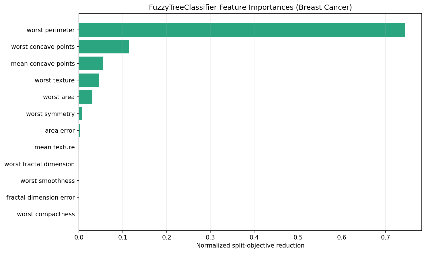
Held-out metrics on one binary and one multiclass tabular dataset.

Breast Cancer: Feature Importance and Local Evidence

Global split-objective importances identify the strongest features; the log-odds waterfall explains one prediction as evidence for the selected class and reports the resulting probability.

Top Breast Cancer feature importances.

Feature contributions to malignant log-odds, converted back to probability in the title.

Iris Multiclass Decision Boundaries

Pairwise Iris feature views with decision regions smoothed from the full fitted model's per-example predictions.

Diagonal panels show per-class feature distributions; off-diagonal panels show connected decision regions interpolated from the full model's predictions on the Iris rows.

Probability Surface

Smooth fuzzy splits produce gradual probability transitions around decision boundaries.

Left: FuzzyTreeClassifier (smooth gradient). Right: DecisionTreeClassifier (step function).

Running the Notebooks

The demo notebooks are in the repository root and generate the charts shown in these docs:

fuzzydtree/
  regressor_demo.ipynb     # FuzzyTreeRegressor examples
  classifier_demo.ipynb    # FuzzyTreeClassifier examples
  docs/
    index.html             # This documentation page
    generate_charts.py     # Run to regenerate all chart images
    img/                   # Generated chart images
      tree_surface_comparison.png
      tree_structure.png
      tree_feature_importances.png
      tree_predicted_vs_actual.png
      tree_explainability_waterfall.png
      classifier_real_benchmarks.png
      classifier_feature_importances.png
      classifier_log_odds_waterfall.png
      classifier_iris_probabilities.png
      classifier_decision_boundaries.png
      classifier_proba_heatmap.png
      classifier_multiclass.png